
Understand and smooth response irregularities
Step by step: understand, predict, adjust and calculate.
01 · Identify the cause first
A peak is a region with too much level. A dip may instead result from lower efficiency, resonance, directivity or cancellation. These causes do not respond identically to a crossover. The demo starts with a deliberately simple synthetic peak. It is not a measurement of a specific driver.
02 · Adjust height, position and width separately
Centre frequency determines where correction acts. Gain determines how much it boosts or cuts. Q determines width. Change only one control at first. A narrow correction in the wrong place can make response less smooth even when the attenuation value looks right.
03 · Active correction and targeted passive attenuation
In the active teaching model, an inverse function exactly compensates the resonant function. A passive crossover cannot add arbitrary energy. A shunt series-resonant circuit provides a low-impedance path near resonance and needs suitable upstream impedance to create attenuation. A parallel-resonant circuit placed in series behaves differently. Load impedance also affects depth and width.
04 · Cancellation is the counterexample
Switch to cancellation. Two equally strong signals with opposing phase can sum to zero. Finite amplification of that same shared signal cannot restore the zero. With real loudspeakers, check polarity, delay, measurement position and reflections. Not every narrow dip should be filled with strong EQ.
05 · Then inspect impedance and loading
A pretty magnitude curve is not enough. Passive components can lower input impedance and dissipate power. Active boosts need voltage and excursion headroom. Check several measurement angles too. A correction that only works on one axis can worsen behaviour in a room.
Workshop takeaway
Measure and understand the cause first, then apply targeted attenuation. The smoothest drawn line is not automatically the best loudspeaker.
Work it out · answers unfold
Write down your prediction first, then your calculation. Open the answer only when you are ready to compare.
01 · RC low-pass: R = 1 kΩ, C = 100 nF. Find cutoff with ideal source and unloaded output across C.
Show worked answer
- RC = 0.0001 s.
- Cutoff = 1/(2πRC).
- Cutoff = 1591.55 Hz.

02 · What voltage ratio and dB value does this low-pass have at cutoff?
Show worked answer
- Ratio = 1/√2 = 0.7071.
- 20 log10(0.7071).
- Result: -3.01 dB.

03 · Find this low-pass voltage ratio at ten times cutoff.
Show worked answer
- Frequency ratio: 10.
- Ratio = 1/√(1 + 10²).
- 0.0995 or -20.04 dB.

04 · You want to halve the RC low-pass cutoff while retaining R. What changes?
Show worked answer
- Cutoff is inversely proportional to C.
- Double capacitance.
- 100 nF becomes 200 nF.

05 · An RC high-pass has R = 10 kΩ and target cutoff 100 Hz. Find C.
Show worked answer
- Rearrange for C.
- C = 1/(2π · 100 · 10000).
- C = 159.15 nF.

06 · An ideal series inductor feeds a purely resistive 8 Ω substitute driver. Target first-order electrical low-pass at 2 kHz. Find L.
Show worked answer
- At cutoff, inductive reactance equals R.
- L = R/(2πfc).
- L = 0.637 mH.

07 · An ideal series capacitor feeds 8 Ω. Target first-order electrical high-pass at 2 kHz. Find C.
Show worked answer
- At cutoff, capacitive reactance magnitude equals R.
- C = 1/(2πfcR).
- C = 9.947 µF.

08 · The substitute driver in task 7 is actually 6 Ω; C is unchanged. What is the electrical cutoff?
Show worked answer
- Cutoff is inversely proportional to R.
- New cutoff = 2000 · 8/6.
- Result: 2666.67 Hz.

09 · A speaker has 8 Ω nominal impedance. Why is task 6 not a complete real crossover design?
Show worked answer
- Impedance varies with frequency and is complex.
- The acoustic driver response also contributes.
- Include measured magnitude, phase and mounting geometry.
10 · A branch should be attenuated by 6 dB in voltage magnitude. Find the ratio.
Show worked answer
- Convert dB back to voltage ratio.
- k = 10^(-6/20).
- k = 0.5012.

11 · Constant-input-resistance L-pad: load 8 Ω, k = 0.5. Find series and shunt resistors. Shunt is across load.
Show worked answer
- Series R = R(1-k) = 4 Ω.
- Shunt R = Rk/(1-k) = 8 Ω.
- 8 Ω parallel 8 Ω = 4 Ω, plus 4 Ω = 8 Ω.

12 · The L-pad in task 11 receives 8 V. Find load power and both resistor dissipations.
Show worked answer
- Source current = 8/8 = 1 A.
- Series resistor: 4 W; output: 4 V.
- Load and shunt resistor each dissipate 2 W.

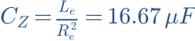
13 · Idealised driver: Re = 6 Ω, Le = 0.6 mH. Find Zobel R and C for the Re-plus-Le model.
Show worked answer
- Zobel R = Re = 6 Ω.
- Zobel C = Le/Re².
- C = 16.67 µF. This model has no mechanical resonance.
14 · Which is correct: a Zobel automatically flattens sound pressure, or it first compensates an impedance rise?
Show worked answer
- First, impedance compensation.
- This can make the preceding crossover behave more predictably.
- Acoustic flatness is not guaranteed.
15 · A series RLC branch has L = 1 mH and C = 10 µF. Find resonance frequency.
Show worked answer
- L · C = 10⁻⁸.
- Square root = 0.0001.
- Resonance = 1591.55 Hz.

16 · How do you move this resonance to half frequency while retaining L?
Show worked answer
- Resonance is inversely proportional to square root of C.
- Quadruple C for half frequency.
- New C = 40 µF.

17 · A measured peak at 2 kHz is 4 dB above target. What voltage ratio is needed for ideal local correction?
Show worked answer
- Correction is -4 dB.
- Ratio = 10^(-4/20).
- Ratio = 0.6310; bandwidth and phase must also fit.

18 · A deep dip comes from opposite-phase sound contributions. Why is strong EQ boost usually a poor first fix?
Show worked answer
- Cancellation remains.
- More drive increases excursion and power.
- First check polarity, delay, geometry and individual branches.
19 · Two ideal acoustic LR4 branches are each -6.02 dB at crossover and in phase. What is their sum?
Show worked answer
- Each branch has pressure ratio 0.5.
- Add in phase: 0.5 + 0.5 = 1.
- Sum = 0 dB.

20 · Plan a fair before-and-after test of a crossover correction. Name four conditions.
Show worked answer
- Same measurement position and excitation.
- Measure branches and sum with timing preserved.
- Check impedance and multiple angles; use identical smoothing.
Further reading
Original teaching models and authored exercises. Sources provide technical background; no manufacturer measurement curves are reproduced.